Market Values Analysis for Housing Units
This project is maintained by TarekDib03
Exploratory Data Analysis and Multi-linear Regression - Market Values for Housing Units
The data sets for the capstone of the Business Statistics and Analysis Specialization, offered by Rice University through the Coursera platform, come from the Housing Affordability Data System of the US Department of Housing and Urban Development. These data sets are generally referred to using the acronym, HADS. This Housing Affordability Data System, or HADS, is a set of housing unit level data sets that aims to study the affordability of housing units, and the housing cost burdens of households, relative to area median incomes, poverty level incomes, and fair market rent. The purpose of this dataset is to provide analysts with consistent measures of affordability and cost burdens over a long period. The data sets are based on the American Housing Survey, AHS, national files from 1985 onwards. Housing-level variables include information on the number of rooms in the housing unit; the year the unit was built; whether it was occupied or vacant; whether the unit was rented or owned; whether it was a single unit or multi-unit structure; the number of units in the building; the current market value of the unit. The dataset also includes variables describing the number of people living in the household, household income, the type of residential area, and other features. The features are defined in a separate section of the report. The data sets are made available to the public by the US Department of Housing and Urban Development. These data are made available every two years. For this project, data from 2005 onwards will be used. That is we will use the data from 2005, 2007, 2009, 2011, and 2013. The data can be downloaded from this link.
The Specialization required using MS Excel. However, I used Python’s multiple modules to process, manipulate, visualize, and analyze data. To build a multi-linear regression model, I used 2 different packages for a learning purpose. Several modules were used in this project: Pandas, Numpy, Seaborn, Matplotlib, Statsmodels, Scipy, Scikit-learn, etc.
Reading Data and Importing Modules
# Change working directory
import os
os.chdir("D:\Rice_Uni_Business_Analytics_Capstone\Data")
# Data files with extension .txt
txt_files = [item for item in os.listdir() if item.endswith(".txt")]
txt_files
['thads2001.txt',
 'thads2003.txt',
 'thads2005.txt',
 'thads2007.txt',
 'thads2009.txt',
 'thads2011.txt',
 'thads2013.txt']
# Columns slected to be used for analysis
usecols = ["CONTROL", "AGE1", "METRO3", "REGION", "LMED", "FMR", "IPOV", "BEDRMS", "BUILT", "STATUS",
           "TYPE", "VALUE", "NUNITS","ROOMS", "PER", "ZINC2", "ZADEQ", "ZSMHC", "STRUCTURETYPE",
           "OWNRENT", "UTILITY", "OTHERCOST", "COST06", "COST08","COST12", "COSTMED", "ASSISTED"]
# Import modules
import pandas as pd
import numpy as np
import seaborn as sns
import matplotlib.pyplot as plt
import statsmodels.api as sm
from statsmodels.stats.outliers_influence import variance_inflation_factor
from statsmodels.formula.api import ols
from scipy import stats
import warnings
data_2001 = pd.read_csv("thads2001.txt", sep=",", usecols=usecols)
data_2003 = pd.read_csv("thads2003.txt", sep=",", usecols=usecols)
data_2005 = pd.read_csv("thads2005.txt", sep=",", usecols=usecols)
data_2007 = pd.read_csv("thads2007.txt", sep=",", usecols=usecols)
data_2009 = pd.read_csv("thads2009.txt", sep=",", usecols=usecols)
data_2011 = pd.read_csv("thads2011.txt", sep=",", usecols=usecols)
data_2013 = pd.read_csv("thads2013.txt", sep=",", usecols=usecols)
Data Manipulation and Statistical Analysis
# Initialize a list
size_list = []
# Iterate over the length of txt_files to append the size of each file to the size_list. Select
# only market values that are $1000 or more
for i in range(len(txt_files)):
    df = pd.read_csv(txt_files[i], sep=",", usecols=usecols)
    df = df[df["VALUE"] >= 1000]
    size_list.append(df.shape[0])
# Print the size of each file as formated below
years = range(2001, 2015, 2)
for i in range(len(txt_files)):
    print("The number of housing units that have market values of $1,000 or more in {} is {}"
          .format(years[i], size_list[i]))
The number of housing units that have market values of $1,000 or more in 2001 is 29381
The number of housing units that have market values of $1,000 or more in 2003 is 33434
The number of housing units that have market values of $1,000 or more in 2005 is 30514
The number of housing units that have market values of $1,000 or more in 2007 is 27785
The number of housing units that have market values of $1,000 or more in 2009 is 31317
The number of housing units that have market values of $1,000 or more in 2011 is 85050
The number of housing units that have market values of $1,000 or more in 2013 is 36675
# Extract the names of the dataframes
def get_df_name(df):
    '''Extract the name of the data frame. Input of the function is the dataframe df'''
    name =[x for x in globals() if globals()[x] is df][0]
    return name
# Change names of the `VALUE` and `STATUS` variables to match the year
def column_name_change(df):
    '''Change the names of the VALUE and STATUS columns. Input is a dataframe'''
    df.rename(columns={"VALUE": "VALUE_{}".format(get_df_name(df)[-4:]),
                       "STATUS": "STATUS_{}".format(get_df_name(df)[-4:]),
                       "FMR": "FMR_{}".format(get_df_name(df)[-4:])}, inplace = True)
# Test
get_df_name(data_2001)
'data_2001'
dfs = [data_2005, data_2007, data_2009, data_2011, data_2013]
for df_name in dfs:
    column_name_change(df_name)
# Now what is the average market value (in $) across all housing units for year 2005
data_2005[data_2005["VALUE_2005"] >= 1000]["VALUE_2005"].mean()
246504.11244019138
# Subsets of the dataframes - market value is $1000 or more
def f(df, x):
    return df[df[x] >= 1000]
# A list of the yearly market value variables
yearly_value = ["VALUE_2005", "VALUE_2007", "VALUE_2009", "VALUE_2011", "VALUE_2013"]
# A list of yearly status
yearly_status = ["STATUS_2005", "STATUS_2007", "STATUS_2009", "STATUS_2011", "STATUS_2013"]
# A list of the dataframes of the years 2005 through 2013
dfs = [data_2005, data_2007, data_2009, data_2011, data_2013]
# Initialize the status list
status = []
# Iterate over the yearly data and group it by status to count the number of occupied vs. vacant apartments in these housing
# units
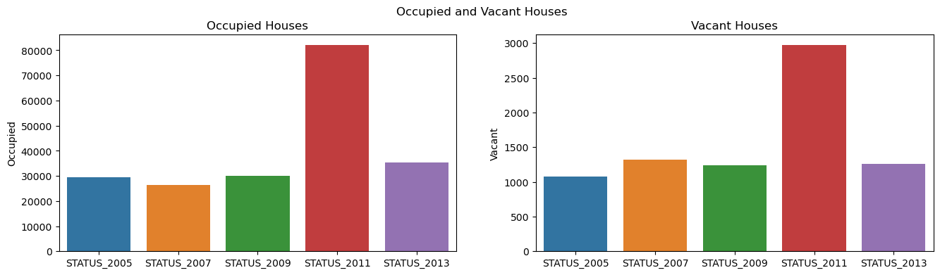
for i in range(len(yearly_value)):
status.append(f(dfs[i], yearly_value[i]).groupby([yearly_status[i]])[yearly_status[i]].count())
# Convert the list to a datafram
status_df = pd.DataFrame(status) # '1': occupied, '3': not occupied
# Rename columns to Occupied and Vacant, respectively
status_df.rename(columns={"'1'": 'Occupied', "'3'": 'Vacant'}, inplace=True)
fig, axes = plt.subplots(1, 2, sharex=True, figsize=(16,4))
fig.suptitle('Occupied and Vacant Houses')
axes[0].set_title('Occupied Houses')
axes[1].set_title('Vacant Houses')
sns.barplot(ax = axes[0], x = status_df.index, y = status_df.Occupied)
sns.barplot(ax = axes[1], x = status_df.index, y = status_df.Vacant)
<Axes: title={'center': 'Vacant Houses'}, ylabel='Vacant'>
# Comparison of the average market value between occupied and vacant housing units
df_2007_sub = f(data_2007[["STATUS_2007", "VALUE_2007"]], "VALUE_2007")
df_2007_sub.groupby("STATUS_2007").mean().round(2)
| VALUE_2007 | |
|---|---|
| STATUS_2007 | |
| '1' | 278960.75 |
| '3' | 289004.49 |
# Standard deviation
df_2007_sub.groupby("STATUS_2007").std().round(2)
| VALUE_2007 | |
|---|---|
| STATUS_2007 | |
| '1' | 317162.77 |
| '3' | 306203.82 |
# Now mean and standard deviation for 2013
df_2013_sub = f(data_2013[["STATUS_2013", "VALUE_2013"]], "VALUE_2013")
print(df_2013_sub.groupby("STATUS_2013").mean().round(2))
print(df_2013_sub.groupby("STATUS_2013").std().round(2))
             VALUE_2013
STATUS_2013
'1'           249858.55
'3'           251996.82
             VALUE_2013
STATUS_2013
'1'           282290.65
'3'           389653.09
# Report the t-statistic from the difference in means test using the 2011 data

# Two-sample independent t-test

# 1. Import stats library from scipy
from scipy import stats

# 2. Prepare data
occupied_2011 = f(data_2011, "VALUE_2011")[f(data_2011, "VALUE_2011")["STATUS_2011"] == "'1'"]["VALUE_2011"]
vacant_2011 = f(data_2011, "VALUE_2011")[f(data_2011, "VALUE_2011")["STATUS_2011"] == "'3'"]["VALUE_2011"]

# 3. Calculate the t-statistic and p-value
t_stat, p_value = stats.ttest_ind(occupied_2011, vacant_2011)
print(round(t_stat, 4), round(p_value, 4))
6.397 0.0
# Now the t-statistic from the difference in means test using the 2013 data
occupied_2013 = f(data_2013, "VALUE_2013")[f(data_2013, "VALUE_2013")["STATUS_2013"] == "'1'"]["VALUE_2013"]
vacant_2013 = f(data_2013, "VALUE_2013")[f(data_2013, "VALUE_2013")["STATUS_2013"] == "'3'"]["VALUE_2013"]

# 3. Calculate the t-statistic and p-value
t_stat_2013, p_value_2013 = stats.ttest_ind(occupied_2013, vacant_2013)
print(round(t_stat_2013, 4), round(p_value_2013, 4))
-0.2599 0.7949
def diff_in_means_test(df, x, y):
    '''Difference in means test for current market values of occupied vs. vacant housing units. The Function f(df, x) is used to
        extract market values that are $1,000 or more.
    Inputs: dataframe df, x: column name (string), y: column name (string)
    '''
    occupied = f(df, x)[f(df, x)[y] == "'1'"][x]
    vacant = f(df, x)[f(df, x)[y] == "'3'"][x]
    t_stat, p_value = stats.ttest_ind(occupied, vacant)
    return round(t_stat, 4), round(p_value, 4)
# Years - use the range function in Python to create a list of values between 2005 and 2013 with a 2-year increment
years_2 = range(2005, 2015, 2)
# Initiate an empty dictionary for the t statistics values
t_stats = {}
# Empty dictionary for the p-values
p_values = {}
# Iterate over the length of the names of dataframes within the list dfs to populate the above dictionaries
for i in range(len(dfs)):
    t_stats[years_2[i]] = diff_in_means_test(dfs[i], yearly_value[i], yearly_status[i])[0]
    p_values[years_2[i]] = diff_in_means_test(dfs[i], yearly_value[i], yearly_status[i])[1]
# Use the Pandas melt method to transpose (unpivot a wide dataframe into a long one) the dataframe
pd.melt(pd.DataFrame([t_stat])).rename(columns={"variable": "Year", "value": "t_stat"})
| Year | t_stat | |
|---|---|---|
| 0 | 0 | 6.397 |
# Same for p-values
pd.melt(pd.DataFrame([p_values])).rename(columns={"variable": "Year", "value": "p_value"})
| Year | p_value | |
|---|---|---|
| 0 | 2005 | 0.0416 |
| 1 | 2007 | 0.2609 |
| 2 | 2009 | 0.8465 |
| 3 | 2011 | 0.0000 |
| 4 | 2013 | 0.7949 |
# Similar to the above diff_in_means function, but the test is one-sided
def one_sided_ttest(df, x, y):
    occupied = f(df, x)[f(df, x)[y] == "'1'"][x]
    vacant = f(df, x)[f(df, x)[y] == "'3'"][x]
    t_stat, p_value = stats.ttest_ind(occupied, vacant, alternative = 'less')
    return round(t_stat, 4), round(p_value, 4)
t_stats_one = {}
p_values_one = {}

for i in range(len(dfs)):
    p_values_one[years_2[i]] = one_sided_ttest(dfs[i], yearly_value[i], yearly_status[i])[1]
pd.melt(pd.DataFrame([p_values_one])).rename(columns={"variable": "Year", "value": "p_value"})
| Year | p_value | |
|---|---|---|
| 0 | 2005 | 0.9792 |
| 1 | 2007 | 0.1305 |
| 2 | 2009 | 0.4232 |
| 3 | 2011 | 1.0000 |
| 4 | 2013 | 0.3975 |
# Merge all the data frames (2005 through 2013)
yearly_fmr = data_2005[["CONTROL", "FMR_2005"]].merge(
    data_2007[["CONTROL", "FMR_2007"]], on="CONTROL").merge(
    data_2009[["CONTROL", "FMR_2009"]], on="CONTROL").merge(
    data_2011[["CONTROL", "FMR_2011"]], on="CONTROL").merge(
    data_2013[["CONTROL", "FMR_2013"]], on="CONTROL")
yearly_fmr.head()
| CONTROL | FMR_2005 | FMR_2007 | FMR_2009 | FMR_2011 | FMR_2013 | |
|---|---|---|---|---|---|---|
| 0 | '100007130148' | 519 | 616 | 685 | 711 | 737 |
| 1 | '100007390148' | 600 | 605 | 670 | 673 | 657 |
| 2 | '100007540148' | 788 | 807 | 897 | 935 | 988 |
| 3 | '100008700141' | 702 | 778 | 743 | 796 | 773 |
| 4 | '100009170148' | 546 | 599 | 503 | 531 | 552 |
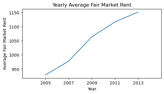
Yearly Average Fair Market Rent
# Initiate an empty list for the fair market rent
fmr_columns = []
warnings.filterwarnings("ignore")
for column in list(yearly_fmr.columns):
    if column.startswith("FMR"):
        fmr_columns.append(column)

yearly_fmr_sub = yearly_fmr

for fmr in fmr_columns:
    yearly_fmr_sub = yearly_fmr_sub[yearly_fmr[fmr] > 0]
yearly_fmr_sub.shape
(26373, 6)
# Test
fmr_min = []
for fmr in fmr_columns:
    fmr_min.append(yearly_fmr_sub[fmr].min())
fmr_min
[360, 387, 427, 424, 421]
fmr_yearly_avgs = []
warnings.filterwarnings("ignore")
for i in range(5):
    fmr_yearly_avgs.append(round(yearly_fmr_sub.describe().loc['mean'][i],2))
fmr_yearly_avgs
[929.04, 977.77, 1063.87, 1116.38, 1151.57]
# Paired ttest
def paired_ttest(x, y):
    t_stat, p_value = stats.ttest_rel(yearly_fmr_sub[x], yearly_fmr_sub[y])
    return round(t_stat, 4), round(p_value, 4)
t_stats_paired = []
p_values_paired = []
fmrs = ["FMR_2005", "FMR_2007", "FMR_2009", "FMR_2011", "FMR_2013"]

for i in range(1, len(fmrs)):
    t_stats_paired.append(paired_ttest(fmrs[i], fmrs[i-1])[0])

t_stats_paired
[69.4904, 124.3222, 74.1512, 58.2109]
# OR
for i in range(1, len(fmrs)):
    print("The t-statistic for the difference in means test for the years {} and {} is {}".
          format(fmrs[i-1][-4:], fmrs[i][-4:], paired_ttest(fmrs[i], fmrs[i-1])[0]))
The t-statistic for the difference in means test for the years 2005 and 2007 is 69.4904
The t-statistic for the difference in means test for the years 2007 and 2009 is 124.3222
The t-statistic for the difference in means test for the years 2009 and 2011 is 74.1512
The t-statistic for the difference in means test for the years 2011 and 2013 is 58.2109
The large values of the t-statistics inform us that there is a significant difference in average fair market rents in subsequent
years. What I mean is that the fair market rent in 2007 is statistically significantly different from that in 2005, 2009 is
significantly different from 2007, etc.

def percent_increase_fmr(x, y):
    ''' The function returns percentage difference in fair market rent in subsequent years (difference between 2005 and 2007,
        between 2007 and 2009, etc.)

        Inputs: x - year, y - next available year
    '''
    return((yearly_fmr_sub[y] - yearly_fmr_sub[x]) / yearly_fmr_sub[x] * 100)
# Iterate over the length of fmrs to output the percentage increase in fair market rent between 2 subsequent years

for i in range(1, len(fmrs)):
    print("The average percent increase in fair market rent between {} and {} is {}%".
          format(fmrs[i-1][-4:], fmrs[i][-4:],
                 round(percent_increase_fmr(fmrs[i-1], fmrs[i]).mean(),2)))
The average percent increase in fair market rent between 2005 and 2007 is 6.21%
The average percent increase in fair market rent between 2007 and 2009 is 9.28%
The average percent increase in fair market rent between 2009 and 2011 is 5.09%
The average percent increase in fair market rent between 2011 and 2013 is 3.77%
# lets draw a line chart for the fair market values for the years 2005 through 2013
years = [2005, 2007, 2009, 2011, 2013]
fmr_yearly_data = pd.DataFrame({"year": years, "avg_yearly_fmr": fmr_yearly_avgs})
fmr_yearly_data
| year | avg_yearly_fmr | |
|---|---|---|
| 0 | 2005 | 929.04 |
| 1 | 2007 | 977.77 |
| 2 | 2009 | 1063.87 |
| 3 | 2011 | 1116.38 |
| 4 | 2013 | 1151.57 |
fig, ax = plt.subplots(figsize=(6, 3))
warnings.filterwarnings("ignore")
sns.lineplot(data = fmr_yearly_data, x = "year", y = "avg_yearly_fmr", ax=ax)
ax.set_xlim(2003,2015)
ax.set_xticks(range(2005,2015,2))
plt.title("Yearly Average Fair Market Rent")
plt.xlabel("Year")
plt.ylabel("Average Fair Market Rent");
fvalue, pvalue = stats.f_oneway(yearly_fmr_sub["FMR_2005"], yearly_fmr_sub["FMR_2007"],
                               yearly_fmr_sub["FMR_2009"], yearly_fmr_sub["FMR_2011"],
                               yearly_fmr_sub["FMR_2013"])
print(fvalue, pvalue)
1706.7912624191479 0.0
Data from 2013 for Linear Regression Analysis - Owned Single Family House Units
Define the Variables used in Remaining Analysis for the Year 2013
- CONTROL Character: A control variable for Housing Unit. Useful to match data across datasets from different years.
- AGE1: Age of head of household
- METRO3 - a character variable with options ‘1’,’2’, ‘3’, ‘4’ or ‘5’ where ‘1’ : Central City, ‘2’, ‘3’, ‘4’, ‘5’ :Others
- REGION Character ‘1’,’2’, ‘3’ or ‘4’. The four census regions—Northeast, Midwest, South, and West.
- LMED (Numerical, $): Area Median Income
- FMR (Numerical, $): Fair Market Monthly Rent
- IPOV (Numerical, $): Poverty Income threshold
- BEDRMS (Numerical): Number of Bedrooms in the unit
- BUILT (Numerical): Year the unit was built
- STATUS (Character) ‘1’, ‘3’ Occupied or Vacant
- TYPE (Numerical): Structure Type
- 1 House, apartment, flat
- 2 Mobile home with no permanent room added
- 3 Mobile home with permanent room added
- 4 HU, in nontransient hotel, motel, etc
- 5 HU, in permanent transient hotel, motel, etc
- 6 HU, in rooming house
- 7 Boat or recreation vehicle
- 9 HU, not specified above
- VALUE (Numerical, $)): Current market value of unit
- NUNITS (Numerical): Number of Units in Building
- ROOMS (Numerical): Number of rooms in the unit
- PER (Numerical): Number of persons in Household
- ZINC2 (Numerical): Annual Household income
- ZADEQ (Character): Adequacy of unit - ‘1’: Adequate, ‘2’: Moderately Inadequate, ‘3’: Severely Inadequate, ‘-6’: Vacant - No information
- ZSMHC (Numerical, $): Monthly housing costs. For renters, housing cost is contract rent plus utility costs. For Owners, the mortgage is not included
- STRUCTURETYPE (Numerical) Structure Type
- 1 Single Family
- 2 2-4 units
- 3 5-19 units
- 4 20-49 units
- 5 50+ units
- 6 Mobile Home
- -9 Not Known
- OWNRENT (Character), ‘1’, ‘2’
- ‘1’: Owner: Owner occupied, vacant for sale, and sold but not occupied.
- ‘2’: Rental: Occupied units rented for cash and without payment of cash rent. Vacant for rent, vacant for rent or sale, and rented but not occupied.
- UTILITY (Numerical $) Monthly utilities cost (gas, oil, electricity, other fuel, trash collection, and water)
- OTHERCOST (Numerical $) Sum of ‘other monthly costs’ such as Home owners’ or renters’ insurance, Land rent (where distinct from unit rent), Condominium fees (where applicable), Other mobile home fees (where applicable).
- COST06 (Numerical $): Monthly mortgage payments assuming 6% interest. This applies only to “Owners”.
- COST08 (Numerical $): Monthly mortgage payments assuming 8% interest. This applies only to “Owners”.
- COST12 (Numerical $): Monthly mortgage payments assuming 12% interest. This applies only to “Owners”.
- COSTMED (Numerical $): Monthly mortgage payments assuming median interest. This applies only to “Owners”.
- ASSISTED (Numerical) Did the housing unit receive some governmental ‘assistance”?
- 0 Not assisted
- 1 Assisted
- -9 Not Known
In the proceeding analysis, only data from 2013 will be used. Owned single family housing units will be considered for the rest of the analysis. The data will be used to build a multiple linear regression model that would predict the current market values of housing units based on a set of explanatory features.
# Read the 2013 into a different dataframe than the one used before
data_2013_df = pd.read_csv("thads2013.txt", sep=",", usecols=usecols)
data_2013_df.shape
(64535, 27)
Data Processing and Manipulation
def owned_single_family_housing(df, x = "VALUE", value=1000, type=1, structure_type=1, owned="'1'"):
    '''The function inputs a dataframe, a variable name x to condition over, with default values
    of value of $1000, type=1 (house), structure_type=1 (single family), and owned house'''
    return df[(df[x] >= value) &
              (df["TYPE"] == type) &
              (df["STRUCTURETYPE"] == structure_type) &
              (df["OWNRENT"] == owned)].reset_index(drop=True)
owned_single_family_housing_df = owned_single_family_housing(data_2013_df)
owned_single_family_housing_df.info()
<class 'pandas.core.frame.DataFrame'>
RangeIndex: 32825 entries, 0 to 32824
Data columns (total 27 columns):
 #   Column         Non-Null Count  Dtype
---  ------         --------------  -----
 0   CONTROL        32825 non-null  object
 1   AGE1           32825 non-null  int64
 2   METRO3         32825 non-null  object
 3   REGION         32825 non-null  object
 4   LMED           32825 non-null  int64
 5   FMR            32825 non-null  int64
 6   IPOV           32825 non-null  int64
 7   BEDRMS         32825 non-null  int64
 8   BUILT          32825 non-null  int64
 9   STATUS         32825 non-null  object
 10  TYPE           32825 non-null  int64
 11  VALUE          32825 non-null  int64
 12  NUNITS         32825 non-null  int64
 13  ROOMS          32825 non-null  int64
 14  PER            32825 non-null  int64
 15  ZINC2          32825 non-null  int64
 16  ZADEQ          32825 non-null  object
 17  ZSMHC          32825 non-null  int64
 18  STRUCTURETYPE  32825 non-null  int64
 19  OWNRENT        32825 non-null  object
 20  UTILITY        32825 non-null  float64
 21  OTHERCOST      32825 non-null  float64
 22  COST06         32825 non-null  float64
 23  COST12         32825 non-null  float64
 24  COST08         32825 non-null  float64
 25  COSTMED        32825 non-null  float64
 26  ASSISTED       32825 non-null  int64
dtypes: float64(6), int64(15), object(6)
memory usage: 6.8+ MB
owned_single_family_housing_df.drop(columns=["TYPE", "STRUCTURETYPE", "OWNRENT"], inplace=True)
# In the METRO3 (metropolitan status) variable, replace '1' with Central City and '2', '3', '4', or '5'
# with Other
import numpy as np
owned_single_family_housing_df["METRO3"] = np.where(owned_single_family_housing_df.METRO3 == "'1'",
                                                   "central_city", "Other")
# STATUS variable: '1': Occupied, '3': Vacant
owned_single_family_housing_df["STATUS"] = np.where(owned_single_family_housing_df.STATUS == "'1'",
                                                   "occupied", "vacant")
owned_single_family_housing_df.replace({"REGION":{"'1'": "Northeast", "'2'": "Midwest",
                                                 "'3'": "South", "'4'": "West"}}, inplace = True)
owned_single_family_housing_df.replace({"ZADEQ":{"'1'": "Adequate", "'2'": "Moderately_inadequate",
                    "'3'": "Severely_inadequate", "'-6'": "Vacant_No_Info"}}, inplace = True)
owned_single_family_housing_df.replace({"ASSISTED":{0:"Not_Assisted", 1:"Assisted", -9:"Not_known"}},
                                        inplace=True)
owned_single_family_housing_df.describe()
| AGE1 | LMED | FMR | IPOV | BEDRMS | BUILT | VALUE | NUNITS | ROOMS | PER | ZINC2 | ZSMHC | UTILITY | OTHERCOST | COST06 | COST12 | COST08 | COSTMED | |
|---|---|---|---|---|---|---|---|---|---|---|---|---|---|---|---|---|---|---|
| count | 32825.000000 | 32825.000000 | 32825.000000 | 32825.000000 | 32825.000000 | 32825.000000 | 3.282500e+04 | 32825.0 | 32825.000000 | 32825.000000 | 3.282500e+04 | 32825.000000 | 32825.000000 | 32825.000000 | 32825.000000 | 32825.000000 | 32825.000000 | 32825.000000 |
| mean | 53.624158 | 68158.426078 | 1277.328835 | 17184.712628 | 3.251942 | 1967.431104 | 2.573874e+05 | 1.0 | 6.730967 | 2.365362 | 8.488523e+04 | 1311.889992 | 245.215319 | 95.374486 | 2051.174528 | 3045.090902 | 2362.079521 | 1836.053536 |
| std | 19.027382 | 12502.711452 | 396.375112 | 6657.658062 | 0.848657 | 26.742731 | 2.826902e+05 | 0.0 | 1.649389 | 2.070924 | 8.565889e+04 | 1087.194787 | 123.231149 | 104.399267 | 1961.990997 | 3051.403698 | 2302.542808 | 1726.568892 |
| min | -9.000000 | 38500.000000 | 421.000000 | -6.000000 | 0.000000 | 1919.000000 | 1.000000e+04 | 1.0 | 2.000000 | -6.000000 | -1.170000e+02 | -6.000000 | 0.000000 | 0.000000 | 66.459547 | 105.075134 | 78.538812 | 58.101678 |
| 25% | 43.000000 | 60060.000000 | 1004.000000 | 13948.000000 | 3.000000 | 1950.000000 | 1.100000e+05 | 1.0 | 6.000000 | 2.000000 | 3.000000e+04 | 550.000000 | 165.000000 | 41.666667 | 1011.974114 | 1428.901605 | 1141.132406 | 919.600112 |
| 50% | 55.000000 | 64810.000000 | 1204.000000 | 15470.000000 | 3.000000 | 1970.000000 | 1.800000e+05 | 1.0 | 7.000000 | 2.000000 | 6.397400e+04 | 1057.000000 | 222.666667 | 70.000000 | 1546.190945 | 2263.760874 | 1770.776233 | 1391.950224 |
| 75% | 66.000000 | 74008.000000 | 1445.000000 | 23401.000000 | 4.000000 | 1990.000000 | 3.000000e+05 | 1.0 | 8.000000 | 4.000000 | 1.092000e+05 | 1740.000000 | 299.000000 | 108.333333 | 2441.455512 | 3624.254012 | 2814.497683 | 2187.058726 |
| max | 93.000000 | 115300.000000 | 3511.000000 | 51635.000000 | 7.000000 | 2013.000000 | 2.520000e+06 | 1.0 | 15.000000 | 20.000000 | 1.061921e+06 | 10667.000000 | 1249.000000 | 2020.916667 | 19261.472577 | 28992.600365 | 22305.447202 | 17155.289494 |
# Numeric fields that each have values less than 0
x = list(owned_single_family_housing_df
                 .describe()
                 .min()[owned_single_family_housing_df.describe().min() <= 0]
                 .index)
print(x)
['AGE1', 'IPOV', 'BEDRMS', 'NUNITS', 'PER', 'ZINC2', 'ZSMHC', 'UTILITY', 'OTHERCOST']
owned_single_family_housing_df = owned_single_family_housing_df[
    (owned_single_family_housing_df[x] > 0).all(axis=1)]
minimums = pd.DataFrame(owned_single_family_housing_df.describe().min())
min_field_vals = minimums.rename(columns={0: "Minimum"}).reset_index().rename(
    columns={"index": "Field"}).sort_values(by = "Minimum")
min_field_vals.reset_index(inplace=True, drop=True)
Now, all the numeric fields have positive values that are 0 or more as shown in the above summary statistics table. All of the numeric fields have a minimum value that is 0 or more.
owned_single_family_housing_df.shape
(30174, 24)
Exploratory Data Analysis
# Descriptive statistics for the outcome variable "VALUE"
value_descriptive_statistics = pd.DataFrame(owned_single_family_housing_df["VALUE"].describe().round(2)).reset_index()
value_descriptive_statistics.rename(columns={"index": "Statistics", "VALUE": "Value"})
| Statistics | Value | |
|---|---|---|
| 0 | count | 30174.00 |
| 1 | mean | 262685.76 |
| 2 | std | 281724.78 |
| 3 | min | 10000.00 |
| 4 | 25% | 120000.00 |
| 5 | 50% | 190000.00 |
| 6 | 75% | 310000.00 |
| 7 | max | 2520000.00 |
value_descriptive_statistics.to_csv("value.csv")
# Summary statistics for categorical variables
owned_single_family_housing_df.describe(include='object')
| CONTROL | METRO3 | REGION | STATUS | ZADEQ | ASSISTED | |
|---|---|---|---|---|---|---|
| count | 30174 | 30174 | 30174 | 30174 | 30174 | 30174 |
| unique | 30174 | 2 | 4 | 1 | 3 | 1 |
| top | '100003130103' | Other | Midwest | occupied | Adequate | Not_known |
| freq | 1 | 23750 | 9015 | 30174 | 29478 | 30174 |
From the table above, all of the remaining 30,174 housing units are occupied. Therefore, the variable STATTUS will not be included in the regression model, because it will not add any information to the final model. In addition, since about 98% (29,478 out of 30,174) of the housing units have adequate space in the response of the Variable ZADEQ, it will not be included in the linear regression model. Therefore the variables STATUS AND ZADEQ will be dropped from the above dataframe.
plt.figure(figsize=(7,3))
sns.boxplot(owned_single_family_housing_df, x='REGION', y='VALUE')
plt.ylabel("Current Market Value ($)")
plt.xlabel("Region")
plt.title("Distribution of Current Market Value Grouped by Region");
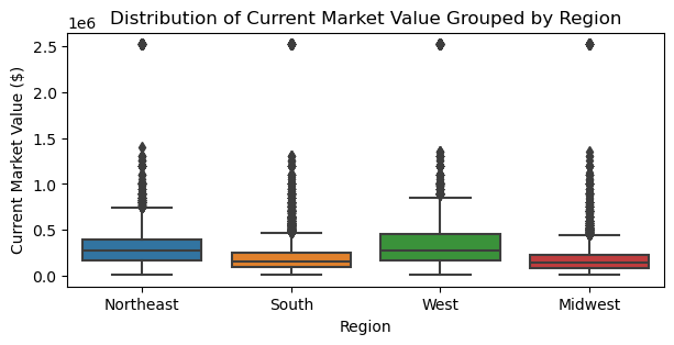
# Average current market value in each region
pd.DataFrame(owned_single_family_housing_df.groupby("REGION")["VALUE"].
             mean().round()).sort_values(by="VALUE").reset_index()
| REGION | VALUE | |
|---|---|---|
| 0 | Midwest | 186871.0 |
| 1 | South | 216831.0 |
| 2 | Northeast | 328229.0 |
| 3 | West | 387586.0 |
All 4 regions have the same maximum market value of $2.52 million, and the same minimum of $10,000. However, the average market value ranges between $186,871 in the Midwest and $387,586 in the West. On average, housing units in the Midwest and South are much cheaper than those in the Northeast and the West.
# Use pivot table to count the number of housing units each year and estimate their market values
tbl = pd.pivot_table(owned_single_family_housing_df, values=["VALUE"],
            index=['BUILT'], aggfunc={"mean", "count"}).reset_index().round()
# Extract the mean and count from the above tbl datafram
units_stats = tbl["VALUE"]
# Rename columns
units_stats.rename(columns={"mean": "yearly_avg_value", "count": "number_of_units"}, inplace=True)
# Concatenate the year to the mean of market values and the count of housing unitrs
units_df = pd.concat([pd.DataFrame(tbl["BUILT"]), units_stats], axis=1)
units_df.rename(columns={"mean": "yearly_avg_value",
                            "count": "number_of_units",
                            "BUILT": "year"}, inplace=True)
units_df.sort_values(by="number_of_units").reset_index(drop=True)
| year | number_of_units | yearly_avg_value | |
|---|---|---|---|
| 0 | 2013 | 13 | 608462.0 |
| 1 | 2011 | 128 | 362969.0 |
| 2 | 2012 | 144 | 355764.0 |
| 3 | 2010 | 169 | 303018.0 |
| 4 | 2009 | 200 | 297150.0 |
| 5 | 2008 | 292 | 356370.0 |
| 6 | 2002 | 376 | 302234.0 |
| 7 | 2000 | 430 | 299395.0 |
| 8 | 2007 | 431 | 300650.0 |
| 9 | 2001 | 443 | 318623.0 |
| 10 | 2003 | 449 | 304321.0 |
| 11 | 2004 | 479 | 274551.0 |
| 12 | 2006 | 483 | 308489.0 |
| 13 | 2005 | 491 | 287515.0 |
| 14 | 1920 | 1121 | 263390.0 |
| 15 | 1930 | 1181 | 261431.0 |
| 16 | 1990 | 1252 | 307388.0 |
| 17 | 1980 | 1393 | 249311.0 |
| 18 | 1940 | 1783 | 231032.0 |
| 19 | 1919 | 1796 | 253207.0 |
| 20 | 1985 | 1846 | 298754.0 |
| 21 | 1970 | 2072 | 245594.0 |
| 22 | 1975 | 2657 | 244212.0 |
| 23 | 1995 | 2861 | 277407.0 |
| 24 | 1960 | 3627 | 242677.0 |
| 25 | 1950 | 4057 | 233823.0 |
units_df.to_csv("year.csv")
From the table above, the yearly average market value barely increases for housing units built between 1940 ($231,032) and 1980 ($249,311). This accounts for a change of only about an 8% increase in market value for housing units built between 1940 and 1980. For those built between 1919 and 1930, the yearly average market values do not seem to change significantly (~3% increase in market values between 1919 and 1930). Housing units built in 1940 have the lowest average market value of about $231,032. The most expensive are housing units built in 2013.
Since there are only 13 housing units built in 2013, and the average market value is almost double the average market value in 2011, housing units built in 2013 will be excluded because the number of units is very low in 2013, and may bias the results!
units_df = units_df[units_df["year"] != 2013]
plt.figure(figsize=(12,5))
sns.barplot(units_df, x='year', y='yearly_avg_value')
plt.title("Average Current Market Values of Units Grouped by Year the Units were built")
plt.ylabel("Avearge Current Market Value of Units");
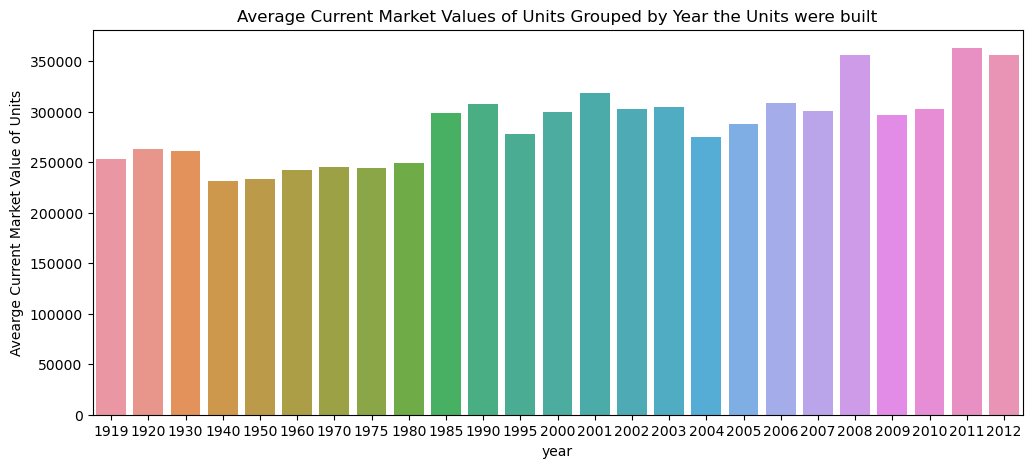
Current average market values for housing units range between $231,032 for those built in 1940 and $362,969 built in 2011, an increase of about 57% in market value in housing units built in 1940. The yearly average market values for housing units built during the global financial crisis (2007 - 2009) fluctuated significantly. For housing units built in 2008, the average market values sit at about \$356,370. However, for housing units built in 2009, the average market values drop significantly to $297,150, i.e. a drop of about 17%. From the above barplot, the average market value is approximately uniformly distributed throughout the years from 1919 to 2012. The average market value per housing unit is estimated to be about $262,686.
# Create the dummy variables for the categorical variables
region_d = pd.get_dummies(owned_single_family_housing_df['REGION'], dtype=int)
metro_d = pd.get_dummies(owned_single_family_housing_df['METRO3'], dtype=int)
adequacy_d = pd.get_dummies(owned_single_family_housing_df['ZADEQ'], dtype=int)
# Concatenate all the dummy variables into one dataframe
d_df = pd.concat([region_d, metro_d, adequacy_d], axis=1)
d_df.head()
| Midwest | Northeast | South | West | Other | central_city | Adequate | Moderately_inadequate | Severely_inadequate | |
|---|---|---|---|---|---|---|---|---|---|
| 0 | 0 | 1 | 0 | 0 | 1 | 0 | 1 | 0 | 0 |
| 1 | 0 | 0 | 1 | 0 | 1 | 0 | 1 | 0 | 0 |
| 2 | 0 | 0 | 1 | 0 | 1 | 0 | 1 | 0 | 0 |
| 3 | 0 | 0 | 1 | 0 | 1 | 0 | 1 | 0 | 0 |
| 4 | 0 | 0 | 1 | 0 | 0 | 1 | 1 | 0 | 0 |
plt.figure(figsize=(5,5))
sns.scatterplot(data = owned_single_family_housing_df,
                x = owned_single_family_housing_df.COST06,
                y = owned_single_family_housing_df.VALUE)
sns.scatterplot(data = owned_single_family_housing_df,
                x = owned_single_family_housing_df.COST08,
                y = owned_single_family_housing_df.VALUE)
sns.scatterplot(data = owned_single_family_housing_df,
                x = owned_single_family_housing_df.COST12,
                y = owned_single_family_housing_df.VALUE)
sns.scatterplot(data = owned_single_family_housing_df,
                x = owned_single_family_housing_df.COSTMED,
                y = owned_single_family_housing_df.VALUE)
#ax.legend(loc='lower ',ncol=4, title="Title")
plt.legend(title='Monthly Mortgage Payments', loc='lower right',
           labels=['6%', '8%', '12%', 'median rate'])
plt.xlabel("Monthly Mortgage Payment")
plt.ylabel("Housing Market Value")
plt.title("Current Market Values of Units vs. Monthly Mortgage Payment");
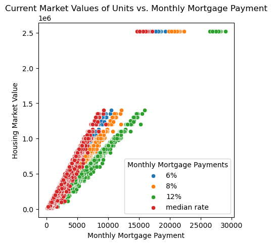
As expected, from the scatterplot above, the higher the monthly mortgage payment, the higher the market values of the housing units. Though this is true, however, for our study, monthly mortgage payments will not add any information to predict the current market value (price) of the housing units. Thus, these variables will not be included in the regression model.
plt.figure(figsize=(6,3))
sns.scatterplot(data=owned_single_family_housing_df, x="BEDRMS", y="ROOMS")
plt.xlabel("Number of Bedrooms")
plt.ylabel("Number of Rooms")
plt.title("Number of Rooms vs. Number of Bedrooms");
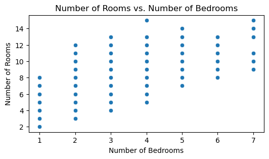
The number of rooms and number of bedrooms are highly correlated as shown in the above scatterplot, and the high correlation between the 2 variables. The Variable BEDRMS will be dropped to avoid multicollinearity issues.
# Create a total_cost variable as follows:
owned_single_family_housing_df["total_cost"] = owned_single_family_housing_df[
    "UTILITY"] + owned_single_family_housing_df[
    "OTHERCOST"] + owned_single_family_housing_df["ZSMHC"]
owned_single_family_housing_df["ln_value"] = np.log(owned_single_family_housing_df.VALUE)
X = owned_single_family_housing_df.drop(columns=["VALUE", "ln_value", "UTILITY", "OTHERCOST", "ZSMHC",
            "UTILITY", "ASSISTED", "CONTROL", "NUNITS", "COST06", "COST08", "COST12", "COSTMED"])
X = pd.concat([X, d_df[['Midwest', 'Northeast', 'South', 'central_city', 'Adequate']]], axis=1)
# Drop the Variables REGION, ZADEQ, METRO3, STATUS
X.drop(columns=["REGION", "ZADEQ", "METRO3", "STATUS"], inplace=True)
X.head()
| AGE1 | LMED | FMR | IPOV | BEDRMS | BUILT | ROOMS | PER | ZINC2 | total_cost | Midwest | Northeast | South | central_city | Adequate | |
|---|---|---|---|---|---|---|---|---|---|---|---|---|---|---|---|
| 0 | 82 | 73738 | 956 | 11067 | 2 | 2006 | 6 | 1 | 18021 | 915.750000 | 0 | 1 | 0 | 0 | 1 |
| 1 | 50 | 55846 | 1100 | 24218 | 4 | 1980 | 6 | 4 | 122961 | 790.666667 | 0 | 0 | 1 | 0 | 1 |
| 2 | 53 | 55846 | 1100 | 15470 | 4 | 1985 | 7 | 2 | 27974 | 1601.500000 | 0 | 0 | 1 | 0 | 1 |
| 3 | 67 | 55846 | 949 | 13964 | 3 | 1985 | 6 | 2 | 32220 | 528.666667 | 0 | 0 | 1 | 0 | 1 |
| 4 | 50 | 60991 | 988 | 18050 | 3 | 1985 | 6 | 3 | 69962 | 1476.000000 | 0 | 0 | 1 | 1 | 1 |
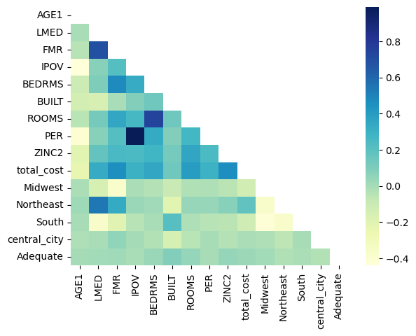
# Correlation Matrix
corr = X.corr()
def highlight_max(s):
    if s.dtype == 'object':
        is_corr = [False for _ in range(s.shape[0])]
    else:
        is_corr = s > 0.5
    return ['color: red;' if cell else 'color:black'
            for cell in is_corr]
corr.style.apply(highlight_max)
| AGE1 | LMED | FMR | IPOV | BEDRMS | BUILT | ROOMS | PER | ZINC2 | total_cost | Midwest | Northeast | South | central_city | Adequate | |
|---|---|---|---|---|---|---|---|---|---|---|---|---|---|---|---|
| AGE1 | 1.000000 | -0.010146 | -0.040166 | -0.440358 | -0.108804 | -0.138537 | -0.046702 | -0.401749 | -0.206399 | -0.237089 | -0.013970 | 0.019804 | 0.000219 | -0.018975 | 0.002276 |
| LMED | -0.010146 | 1.000000 | 0.683971 | 0.078243 | 0.100760 | -0.158059 | 0.123096 | 0.077243 | 0.172790 | 0.329919 | -0.152054 | 0.541857 | -0.372614 | -0.007961 | 0.007868 |
| FMR | -0.040166 | 0.683971 | 1.000000 | 0.216047 | 0.478068 | -0.009525 | 0.349391 | 0.218579 | 0.248834 | 0.456375 | -0.380552 | 0.330926 | -0.197852 | 0.052698 | 0.017112 |
| IPOV | -0.440358 | 0.078243 | 0.216047 | 1.000000 | 0.329640 | 0.088701 | 0.259868 | 0.989618 | 0.242891 | 0.299183 | -0.014878 | 0.034332 | -0.043398 | 0.004929 | -0.005402 |
| BEDRMS | -0.108804 | 0.100760 | 0.478068 | 0.329640 | 1.000000 | 0.141762 | 0.744225 | 0.333674 | 0.276075 | 0.350501 | -0.034834 | 0.013665 | -0.007476 | -0.031947 | 0.031496 |
| BUILT | -0.138537 | -0.158059 | -0.009525 | 0.088701 | 0.141762 | 1.000000 | 0.142026 | 0.088280 | 0.126572 | 0.141853 | -0.089905 | -0.207186 | 0.212904 | -0.151060 | 0.089468 |
| ROOMS | -0.046702 | 0.123096 | 0.349391 | 0.259868 | 0.744225 | 0.142026 | 1.000000 | 0.268147 | 0.353855 | 0.401176 | -0.021500 | 0.037715 | -0.016843 | -0.048646 | 0.043317 |
| PER | -0.401749 | 0.077243 | 0.218579 | 0.989618 | 0.333674 | 0.088280 | 0.268147 | 1.000000 | 0.242559 | 0.292750 | -0.015877 | 0.035158 | -0.043685 | 0.000784 | -0.003385 |
| ZINC2 | -0.206399 | 0.172790 | 0.248834 | 0.242891 | 0.276075 | 0.126572 | 0.353855 | 0.242559 | 1.000000 | 0.462820 | -0.049765 | 0.074081 | -0.052341 | -0.034424 | 0.045125 |
| total_cost | -0.237089 | 0.329919 | 0.456375 | 0.299183 | 0.350501 | 0.141853 | 0.401176 | 0.292750 | 0.462820 | 1.000000 | -0.131444 | 0.180337 | -0.111354 | -0.013059 | 0.026506 |
| Midwest | -0.013970 | -0.152054 | -0.380552 | -0.014878 | -0.034834 | -0.089905 | -0.021500 | -0.015877 | -0.049765 | -0.131444 | 1.000000 | -0.371976 | -0.422289 | -0.016145 | 0.009619 |
| Northeast | 0.019804 | 0.541857 | 0.330926 | 0.034332 | 0.013665 | -0.207186 | 0.037715 | 0.035158 | 0.074081 | 0.180337 | -0.371976 | 1.000000 | -0.368684 | -0.059059 | -0.022263 |
| South | 0.000219 | -0.372614 | -0.197852 | -0.043398 | -0.007476 | 0.212904 | -0.016843 | -0.043685 | -0.052341 | -0.111354 | -0.422289 | -0.368684 | 1.000000 | 0.000810 | -0.010960 |
| central_city | -0.018975 | -0.007961 | 0.052698 | 0.004929 | -0.031947 | -0.151060 | -0.048646 | 0.000784 | -0.034424 | -0.013059 | -0.016145 | -0.059059 | 0.000810 | 1.000000 | -0.029027 |
| Adequate | 0.002276 | 0.007868 | 0.017112 | -0.005402 | 0.031496 | 0.089468 | 0.043317 | -0.003385 | 0.045125 | 0.026506 | 0.009619 | -0.022263 | -0.010960 | -0.029027 | 1.000000 |
# From the correlation matrix above let's drop variables with correlation values greater than 0.5
X_cleaned = X.drop(columns=["BEDRMS"])
corr.to_csv("correlation.csv")
# Empirical distribution of the Variable "VALUE"
warnings.filterwarnings("ignore")
val = sns.displot(data=owned_single_family_housing_df, x='VALUE', height=3, aspect=0.8,
            kde=True, col="REGION")
val.set_axis_labels("Market Value ($)", "Number of Units")
val.set_titles("{col_name} Region");
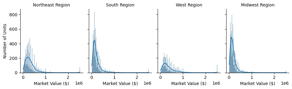
The distribution of VALUE is right skewed. A log transformation could help to make the distribution more bell-shaped!
LNVALUE = np.log(owned_single_family_housing_df.VALUE)
owned_single_family_housing_df['ln_value'] = LNVALUE
warnings.filterwarnings("ignore")
ln_val = sns.displot(data = owned_single_family_housing_df, x='ln_value', height=3, aspect=0.8,
            kde=True, col="REGION")
ln_val.set_axis_labels("Ln(VALUE)", "Number of Units")
ln_val.set_titles("{col_name} Region");
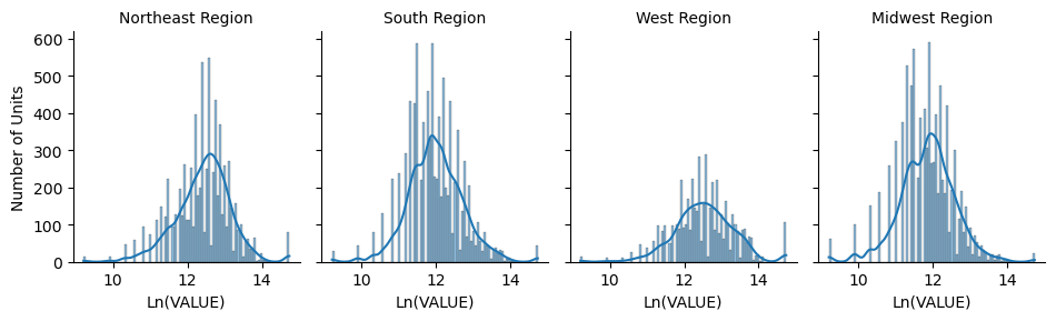
After transformation, the data became normally distributed with equal mean and median of 12, and standard variation of 1. Also the distribution curve above shaow that the ln_value variable is normally distributed. Thus, we will use the transformed variable ln_value to build the linear regression model.
# lower triangular matrix
mask = np.triu(np.ones_like(X.corr()))
warnings.filterwarnings("ignore")
# plotting a triangle correlation heatmap
sns.heatmap(X.corr(), cmap="YlGnBu", annot=True, fmt='0.1f', mask=mask);
Linear Regression Model
y = owned_single_family_housing_df["VALUE"]
X_new = sm.add_constant(X_cleaned)
# Create the linear model
model = sm.OLS(y, X_new)
# Fit the model
results = model.fit()
# Print out the summary of the model results
results.summary()
| Dep. Variable: | VALUE | R-squared: | 0.470 |
|---|---|---|---|
| Model: | OLS | Adj. R-squared: | 0.469 |
| Method: | Least Squares | F-statistic: | 1908. |
| Date: | Sun, 14 Jan 2024 | Prob (F-statistic): | 0.00 |
| Time: | 21:46:13 | Log-Likelihood: | -4.1189e+05 |
| No. Observations: | 30174 | AIC: | 8.238e+05 |
| Df Residuals: | 30159 | BIC: | 8.239e+05 |
| Df Model: | 14 | ||
| Covariance Type: | nonrobust |
| coef | std err | t | P>|t| | [0.025 | 0.975] | |
|---|---|---|---|---|---|---|
| const | 1.79e+05 | 9.79e+04 | 1.828 | 0.068 | -1.29e+04 | 3.71e+05 |
| AGE1 | 2136.8019 | 90.752 | 23.546 | 0.000 | 1958.925 | 2314.679 |
| LMED | -0.0122 | 0.160 | -0.076 | 0.939 | -0.325 | 0.301 |
| FMR | 126.7216 | 5.442 | 23.285 | 0.000 | 116.055 | 137.388 |
| IPOV | -9.6768 | 1.463 | -6.615 | 0.000 | -12.544 | -6.809 |
| BUILT | -186.8934 | 48.683 | -3.839 | 0.000 | -282.314 | -91.473 |
| ROOMS | 1.391e+04 | 869.253 | 15.999 | 0.000 | 1.22e+04 | 1.56e+04 |
| PER | 2.043e+04 | 5991.085 | 3.411 | 0.001 | 8692.119 | 3.22e+04 |
| ZINC2 | 0.4793 | 0.016 | 29.941 | 0.000 | 0.448 | 0.511 |
| total_cost | 114.3134 | 1.295 | 88.272 | 0.000 | 111.775 | 116.852 |
| Midwest | -7.526e+04 | 4435.001 | -16.969 | 0.000 | -8.4e+04 | -6.66e+04 |
| Northeast | -7.382e+04 | 4405.075 | -16.759 | 0.000 | -8.25e+04 | -6.52e+04 |
| South | -6.273e+04 | 4019.413 | -15.607 | 0.000 | -7.06e+04 | -5.49e+04 |
| central_city | -1.036e+04 | 2959.067 | -3.502 | 0.000 | -1.62e+04 | -4562.801 |
| Adequate | 1.349e+04 | 7918.202 | 1.703 | 0.089 | -2034.515 | 2.9e+04 |
| Omnibus: | 30606.729 | Durbin-Watson: | 1.914 |
|---|---|---|---|
| Prob(Omnibus): | 0.000 | Jarque-Bera (JB): | 2336359.516 |
| Skew: | 4.978 | Prob(JB): | 0.00 |
| Kurtosis: | 44.943 | Cond. No. | 1.14e+07 |
Notes:
[1] Standard Errors assume that the covariance matrix of the errors is correctly specified.
[2] The condition number is large, 1.14e+07. This might indicate that there are
strong multicollinearity or other numerical problems.
# Remove variables that may cause a multicollinearity issue
X_reduced = X.drop(columns=["BEDRMS"])
# VIF dataframe
vif_data_2 = pd.DataFrame()
vif_data_2["feature"] = X_reduced.columns

# calculating VIF for each feature
vif_data_2["VIF"] = [variance_inflation_factor(X_reduced.values, i)
                          for i in range(len(X_reduced.columns))]

print(vif_data_2)
         feature         VIF
0           AGE1   18.989908
1           LMED   87.123319
2            FMR   38.378476
3           IPOV  528.409464
4          BUILT  220.863768
5          ROOMS   26.359082
6            PER  228.799280
7          ZINC2    2.869590
8     total_cost    5.239554
9        Midwest    4.144784
10     Northeast    3.330547
11         South    3.414944
12  central_city    1.293290
13      Adequate   43.886523
X_reduced["ln_total_cost"] = np.log(X_reduced.total_cost)
X_reduced["sqrt_ZINC2"] = np.sqrt(X_reduced.ZINC2)
X_reduced["ln_lmed"] = np.log(X_reduced.LMED)
X_reduced["ln_fmr"] = np.log(X_reduced.FMR)
X_reduced["ln_ipov"] = np.log(X_reduced.IPOV)
X_reduced_cleaned = X_reduced.drop(columns=["total_cost", "ZINC2", "LMED", "FMR", "IPOV"])
X_reduced_cleaned.head()
| AGE1 | BUILT | ROOMS | PER | Midwest | Northeast | South | central_city | Adequate | ln_total_cost | sqrt_ZINC2 | ln_lmed | ln_fmr | ln_ipov | |
|---|---|---|---|---|---|---|---|---|---|---|---|---|---|---|
| 0 | 82 | 2006 | 6 | 1 | 0 | 1 | 0 | 0 | 1 | 6.819743 | 134.242318 | 11.208274 | 6.862758 | 9.311723 |
| 1 | 50 | 1980 | 6 | 4 | 0 | 0 | 1 | 0 | 1 | 6.672876 | 350.657953 | 10.930353 | 7.003065 | 10.094851 |
| 2 | 53 | 1985 | 7 | 2 | 0 | 0 | 1 | 0 | 1 | 7.378696 | 167.254297 | 10.930353 | 7.003065 | 9.646658 |
| 3 | 67 | 1985 | 6 | 2 | 0 | 0 | 1 | 0 | 1 | 6.270358 | 179.499304 | 10.930353 | 6.855409 | 9.544238 |
| 4 | 50 | 1985 | 6 | 3 | 0 | 0 | 1 | 1 | 1 | 7.297091 | 264.503308 | 11.018482 | 6.895683 | 9.800901 |
y = owned_single_family_housing_df["ln_value"]
X_reduced_new = sm.add_constant(X_reduced_cleaned)
# Create the linear model
model_reduced = sm.OLS(y, X_reduced_new)
# Fit the model
results_reduced = model_reduced.fit()
# Print out the summary of the model results
results_reduced.summary()
| Dep. Variable: | ln_value | R-squared: | 0.544 |
|---|---|---|---|
| Model: | OLS | Adj. R-squared: | 0.544 |
| Method: | Least Squares | F-statistic: | 2573. |
| Date: | Sun, 14 Jan 2024 | Prob (F-statistic): | 0.00 |
| Time: | 21:46:14 | Log-Likelihood: | -23919. |
| No. Observations: | 30174 | AIC: | 4.787e+04 |
| Df Residuals: | 30159 | BIC: | 4.799e+04 |
| Df Model: | 14 | ||
| Covariance Type: | nonrobust |
| coef | std err | t | P>|t| | [0.025 | 0.975] | |
|---|---|---|---|---|---|---|
| const | 0.1251 | 0.682 | 0.183 | 0.854 | -1.211 | 1.462 |
| AGE1 | 0.0068 | 0.000 | 26.339 | 0.000 | 0.006 | 0.007 |
| BUILT | 0.0026 | 0.000 | 20.218 | 0.000 | 0.002 | 0.003 |
| ROOMS | 0.0667 | 0.002 | 28.952 | 0.000 | 0.062 | 0.071 |
| PER | 0.0469 | 0.012 | 3.792 | 0.000 | 0.023 | 0.071 |
| Midwest | -0.3301 | 0.012 | -28.660 | 0.000 | -0.353 | -0.307 |
| Northeast | -0.1729 | 0.011 | -15.331 | 0.000 | -0.195 | -0.151 |
| South | -0.2409 | 0.010 | -23.158 | 0.000 | -0.261 | -0.221 |
| central_city | -0.0811 | 0.008 | -10.501 | 0.000 | -0.096 | -0.066 |
| Adequate | 0.1372 | 0.021 | 6.648 | 0.000 | 0.097 | 0.178 |
| ln_total_cost | 0.5033 | 0.007 | 75.331 | 0.000 | 0.490 | 0.516 |
| sqrt_ZINC2 | 0.0012 | 3.06e-05 | 39.636 | 0.000 | 0.001 | 0.001 |
| ln_lmed | 0.3095 | 0.029 | 10.507 | 0.000 | 0.252 | 0.367 |
| ln_fmr | 0.4461 | 0.019 | 23.185 | 0.000 | 0.408 | 0.484 |
| ln_ipov | -0.4627 | 0.061 | -7.583 | 0.000 | -0.582 | -0.343 |
| Omnibus: | 2465.572 | Durbin-Watson: | 1.851 |
|---|---|---|---|
| Prob(Omnibus): | 0.000 | Jarque-Bera (JB): | 9572.312 |
| Skew: | -0.345 | Prob(JB): | 0.00 |
| Kurtosis: | 5.672 | Cond. No. | 4.42e+05 |
Notes:
[1] Standard Errors assume that the covariance matrix of the errors is correctly specified.
[2] The condition number is large, 4.42e+05. This might indicate that there are
strong multicollinearity or other numerical problems.
Analysis of Variance
# Ordinary Least Squares (OLS) model
model_aov = ols('ln_value ~ C(REGION)', data = owned_single_family_housing_df).fit()
anova_table = sm.stats.anova_lm(model_aov, typ=2)
anova_table
| sum_sq | df | F | PR(>F) | |
|---|---|---|---|---|
| C(REGION) | 2305.719476 | 3.0 | 1395.326198 | 0.0 |
| Residual | 16618.230365 | 30170.0 | NaN | NaN |
# Independent ttest by Region
region_northwest = owned_single_family_housing_df[owned_single_family_housing_df.REGION=="Northeast"]["VALUE"]
region_west = owned_single_family_housing_df[owned_single_family_housing_df.REGION=="West"]["VALUE"]
region_south = owned_single_family_housing_df[owned_single_family_housing_df.REGION=="South"]["VALUE"]
region_midwest = owned_single_family_housing_df[owned_single_family_housing_df.REGION=="Midwest"]["VALUE"]
res_region = stats.tukey_hsd(region_northwest, region_west, region_south, region_midwest)
type(res_region)
scipy.stats._hypotests.TukeyHSDResult
Using the Tukey HSD test, all the means of current market values are different throughout all 4 regions as shown in the table above. P-values of all groups are close to zero, and thus the null hypothesis is rejected. The null hypothesis claims that the means between the two groups are equal.
Summary Tables
pd.pivot_table(owned_single_family_housing_df, values=["IPOV", "VALUE", "LMED", "FMR",
            "total_cost", "ZINC2", "ROOMS", "PER", "ln_value"],
               index=['REGION']).round(2).sort_values(by="VALUE").reset_index()
| REGION | FMR | IPOV | LMED | PER | ROOMS | VALUE | ZINC2 | ln_value | total_cost | |
|---|---|---|---|---|---|---|---|---|---|---|
| 0 | Midwest | 1053.29 | 17654.28 | 65497.60 | 2.62 | 6.73 | 186870.77 | 84145.04 | 11.86 | 1502.39 |
| 1 | South | 1163.39 | 17390.63 | 61205.95 | 2.55 | 6.74 | 216831.41 | 83743.34 | 12.00 | 1536.89 |
| 2 | Northeast | 1515.51 | 18148.62 | 80309.21 | 2.74 | 6.90 | 328229.01 | 101913.84 | 12.44 | 2113.13 |
| 3 | West | 1585.94 | 18227.47 | 68912.90 | 2.76 | 6.80 | 387585.92 | 98622.69 | 12.54 | 1984.33 |
# Compare the mean and median of the market value of unit befor and after the log transformation
pd.pivot_table(owned_single_family_housing_df, values=["VALUE", "ln_value"], index=['REGION'],
              aggfunc = {"ln_value": ["mean", "median"],
                         "VALUE": ["mean", "median"]}).round(2).reset_index()
| REGION | VALUE | ln_value | |||
|---|---|---|---|---|---|
| mean | median | mean | median | ||
| 0 | Midwest | 186870.77 | 150000.0 | 11.86 | 11.92 |
| 1 | Northeast | 328229.01 | 270000.0 | 12.44 | 12.51 |
| 2 | South | 216831.41 | 160000.0 | 12.00 | 11.98 |
| 3 | West | 387585.92 | 280000.0 | 12.54 | 12.54 |
Mean and median are approximately equal throughout the 4 regions after the Variable VALUE was log-transformed. However, before it was transformed, the mean and median seemed to be significantly different, which implies that current market values of housing units are right-skewed in this case since means are higher than medians.
Use Scikitlearn to run the above Regression Analysis
Importing Required Packages
from sklearn.model_selection import train_test_split
from sklearn.linear_model import LinearRegression
import sklearn.metrics as metrics
y = owned_single_family_housing_df["ln_value"]
# Sperate train and test data
X_train, X_test, y_train, y_test = train_test_split(X_reduced_cleaned, y, test_size = 0.2, random_state=42)
print("The number of samples in train set is {}".format(X_train.shape[0]))
print("The number of samples in test set is {}".format(X_test.shape[0]))
The number of samples in train set is 24139
The number of samples in test set is 6035
# (1) Initiate the model
lr = LinearRegression()
# (2) Fit the model
lr.fit(X_train, y_train)
# (3) Score the model
lr.score(X_test, y_test)
0.5287333822667113
# Coefficients
lr.coef_
array([ 0.00684111,  0.00239845,  0.06792728,  0.04411304, -0.33905494,
       -0.17960855, -0.24822985, -0.08106516,  0.14785642,  0.50224208,
        0.00123396,  0.29875615,  0.44772303, -0.44009229])
# Intercept
lr.intercept_
0.3579597451082446
# Predict
y_pred = lr.predict(X_test)
# Mean Square error
mse = metrics.mean_squared_error(y_test, y_pred)
print("Mean Squared Error {}".format(mse))
Mean Squared Error 0.2888147061037005
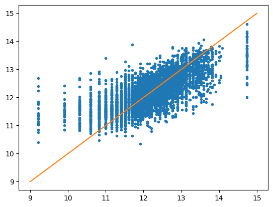
plt.plot(y_test, y_pred, '.')
# plot a line
x = np.linspace(9, 15, 50)
y = x
plt.plot(x, y);
params = np.append(lr.intercept_, lr.coef_)
params
array([ 0.35795975,  0.00684111,  0.00239845,  0.06792728,  0.04411304,
       -0.33905494, -0.17960855, -0.24822985, -0.08106516,  0.14785642,
        0.50224208,  0.00123396,  0.29875615,  0.44772303, -0.44009229])
new_X = np.append(np.ones((len(X_test), 1)), X_test, axis=1)
new_X[0]
array([1.00000000e+00, 5.50000000e+01, 1.95000000e+03, 9.00000000e+00,
       2.00000000e+00, 1.00000000e+00, 0.00000000e+00, 0.00000000e+00,
       0.00000000e+00, 1.00000000e+00, 7.31366473e+00, 2.46752913e+02,
       1.09685258e+01, 7.01121399e+00, 9.64549372e+00])
MSE = (sum((y_test - y_pred)**2)) / (len(new_X) - len(new_X[0]))
MSE
0.28953434407571965
v_b = MSE*(np.linalg.inv(np.dot(new_X.T, new_X)).diagonal())
v_b
array([2.05849036e+00, 3.25093365e-07, 8.29152794e-08, 2.68055427e-05,
       6.20237000e-04, 6.82132546e-04, 6.50615557e-04, 5.45439704e-04,
       3.05842417e-04, 2.27099509e-03, 2.26989324e-04, 4.71487291e-09,
       4.45108265e-03, 1.90402779e-03, 1.53447322e-02])
se = np.sqrt(v_b)
se
array([1.43474400e+00, 5.70169593e-04, 2.87950134e-04, 5.17740695e-03,
       2.49045578e-02, 2.61176673e-02, 2.55071668e-02, 2.33546506e-02,
       1.74883509e-02, 4.76549587e-02, 1.50661649e-02, 6.86649322e-05,
       6.67164347e-02, 4.36351668e-02, 1.23873856e-01])
t_b = params/se
t_b
array([  0.24949381,  11.99837366,   8.32938418,  13.1199431 ,
         1.77128381, -12.98182317,  -7.04149338, -10.6287118 ,
        -4.63538035,   3.10264492,  33.33576166,  17.97080166,
         4.47799939,  10.26060092,  -3.55274553])
p_val = [2*(1 - stats.t.cdf(np.abs(i), (len(new_X) - len(new_X[0])))) for i in t_b]
p_val = np.round(p_val, 3)
p_val
array([0.803, 0.   , 0.   , 0.   , 0.077, 0.   , 0.   , 0.   , 0.   ,
       0.002, 0.   , 0.   , 0.   , 0.   , 0.   ])
2011 Explanatory Variables and 2013 Market Value Variable
- Data from 2011 and 2013 will be merged;
- The Variable
VALUE(market value of housing units) from 2013 is the response variable; - Explanatory variables and the market value variable (
VALUE) from 2011 will be used to build the regression model. This way, the market value from 2011 will contribute to predict the market value in 2013; - Data will be split - 1,000 observations will be held for testing and evaluating the model;
# Reread the datasets
data_2011 = pd.read_csv("thads2011.txt", sep=",", usecols=usecols)
data_2013 = pd.read_csv("thads2013.txt", sep=",", usecols=usecols)
df_merged_2011_2013 = data_2011.merge(data_2013[["CONTROL", "VALUE"]], on = "CONTROL")
df_merged_2011_2013.shape
(46381, 28)
# Rename VALUE_x and VALUE_y according to the year
df_merged_2011_2013.rename(columns={"VALUE_x": "VALUE_2011", "VALUE_y": "VALUE_2013"}, inplace=True)
# Keep VALUE_2011 and VALUE_2013 that are $1000 or more
df_merged_2011_2013_sub = df_merged_2011_2013[(df_merged_2011_2013["VALUE_2011"]>= 1000) & (df_merged_2011_2013["VALUE_2013"]>= 1000)]
df_merged_2011_2013_sub.shape
(24657, 28)
# Owned single family housing units
owned_single_family_units = df_merged_2011_2013_sub[(df_merged_2011_2013_sub.TYPE==1) & (df_merged_2011_2013_sub.STRUCTURETYPE==1) & (df_merged_2011_2013_sub.OWNRENT=="'1'")]
owned_single_family_units.shape
(22232, 28)
owned_single_family_units_df1 = owned_single_family_units.drop(columns=["CONTROL", "TYPE", "STRUCTURETYPE", "COST06", "COST12",
                                            "COST08", "COSTMED", "OWNRENT", "NUNITS", "ASSISTED", "STATUS", "ZSMHC"])
owned_single_family_units_df1.columns
Index(['AGE1', 'METRO3', 'REGION', 'LMED', 'FMR', 'IPOV', 'PER', 'ZINC2',
       'ZADEQ', 'BEDRMS', 'BUILT', 'VALUE_2011', 'ROOMS', 'UTILITY',
       'OTHERCOST', 'VALUE_2013'],
      dtype='object')
# Keep only positive values fore the variables "AGE1", "IPOV", etc.
owned_single_family_units_df2 = owned_single_family_units_df1[(
    owned_single_family_units_df1.AGE1>0) & (
    owned_single_family_units_df1.IPOV>0) & (
    owned_single_family_units_df1.PER>0) & (
    owned_single_family_units_df1.ZINC2>0) & (
    owned_single_family_units_df1.UTILITY>0) & (
    owned_single_family_units_df1.OTHERCOST>0)
].reset_index(drop=True)
owned_single_family_units_df2.head()
| AGE1 | METRO3 | REGION | LMED | FMR | IPOV | PER | ZINC2 | ZADEQ | BEDRMS | BUILT | VALUE_2011 | ROOMS | UTILITY | OTHERCOST | VALUE_2013 | |
|---|---|---|---|---|---|---|---|---|---|---|---|---|---|---|---|---|
| 0 | 40 | '5' | '3' | 55770 | 1003 | 11572 | 1 | 44982 | '1' | 4 | 1980 | 125000 | 8 | 220.500000 | 41.666667 | 130000 |
| 1 | 65 | '5' | '3' | 55770 | 895 | 13403 | 2 | 36781 | '1' | 3 | 1985 | 250000 | 5 | 230.000000 | 40.333333 | 200000 |
| 2 | 48 | '1' | '3' | 62084 | 935 | 17849 | 3 | 57446 | '1' | 3 | 1985 | 169000 | 6 | 236.333333 | 108.333333 | 260000 |
| 3 | 58 | '5' | '4' | 53995 | 1224 | 14895 | 2 | 129964 | '1' | 3 | 1985 | 140000 | 7 | 217.666667 | 55.000000 | 170000 |
| 4 | 57 | '5' | '3' | 55770 | 895 | 14849 | 2 | 258664 | '1' | 3 | 1985 | 225000 | 5 | 187.000000 | 45.833333 | 230000 |
owned_single_family_units_df2.shape
(20821, 16)
# Log-transform a number of explanatory variables and the response variable "VALUE_2013"
variables = owned_single_family_units_df2[["LMED", "ZINC2", "FMR", "UTILITY", "OTHERCOST","VALUE_2011", "VALUE_2013"]]
features_transformed = np.log(variables)
features_transformed.tail()
| LMED | ZINC2 | FMR | UTILITY | OTHERCOST | VALUE_2011 | VALUE_2013 | |
|---|---|---|---|---|---|---|---|
| 20816 | 11.138348 | 11.512385 | 7.029088 | 5.468763 | 3.624341 | 11.918391 | 12.206073 |
| 20817 | 11.018629 | 9.862666 | 6.698268 | 5.335934 | 4.335110 | 12.388394 | 12.429216 |
| 20818 | 11.018629 | 10.735222 | 7.074117 | 5.542243 | 3.555348 | 11.849398 | 11.918391 |
| 20819 | 11.018629 | 10.125190 | 7.255591 | 5.519793 | 3.314186 | 11.608236 | 12.301383 |
| 20820 | 11.018629 | 9.902587 | 7.074117 | 6.080696 | 3.912023 | 11.849398 | 12.388394 |
# Drop the above columns from the owned_single_family_units_df2 dataframe then concatenate the above transformed dataframe to it
cols = ["LMED", "ZINC2", "FMR", "IPOV", "UTILITY", "OTHERCOST", "VALUE_2011", "VALUE_2013"]
owned_single_family_units_df3 = owned_single_family_units_df2.drop(columns = cols)
owned_single_family_units_df4 = pd.concat([owned_single_family_units_df3, features_transformed], axis=1)
owned_single_family_units_df4.head()
| AGE1 | METRO3 | REGION | PER | ZADEQ | BEDRMS | BUILT | ROOMS | LMED | ZINC2 | FMR | UTILITY | OTHERCOST | VALUE_2011 | VALUE_2013 | |
|---|---|---|---|---|---|---|---|---|---|---|---|---|---|---|---|
| 0 | 40 | '5' | '3' | 1 | '1' | 4 | 1980 | 8 | 10.928991 | 10.714018 | 6.910751 | 5.395898 | 3.729701 | 11.736069 | 11.775290 |
| 1 | 65 | '5' | '3' | 2 | '1' | 3 | 1985 | 5 | 10.928991 | 10.512737 | 6.796824 | 5.438079 | 3.697178 | 12.429216 | 12.206073 |
| 2 | 48 | '1' | '3' | 3 | '1' | 3 | 1985 | 6 | 11.036244 | 10.958601 | 6.840547 | 5.465243 | 4.685213 | 12.037654 | 12.468437 |
| 3 | 58 | '5' | '4' | 2 | '1' | 3 | 1985 | 7 | 10.896647 | 11.775013 | 7.109879 | 5.382965 | 4.007333 | 11.849398 | 12.043554 |
| 4 | 57 | '5' | '3' | 2 | '1' | 3 | 1985 | 5 | 10.928991 | 12.463285 | 6.796824 | 5.231109 | 3.825012 | 12.323856 | 12.345835 |
# Replace codes with the corresponding value
owned_single_family_units_df4.replace({"REGION":{"'1'": "Northeast", "'2'": "Midwest",
                                                 "'3'": "South", "'4'": "West"}}, inplace = True)
owned_single_family_units_df4["METRO3"] = np.where(owned_single_family_units_df4.METRO3 == "'1'",
                                                   "Metro", "Other")
owned_single_family_units_df4.replace({"ZADEQ":{"'1'": "Adequate", "'2'": "Moderately_inadequate",
                    "'3'": "Severely_inadequate", "'-6'": "Vacant_No_Info"}}, inplace = True)
owned_single_family_units_df4.tail()
| AGE1 | METRO3 | REGION | PER | ZADEQ | BEDRMS | BUILT | ROOMS | LMED | ZINC2 | FMR | UTILITY | OTHERCOST | VALUE_2011 | VALUE_2013 | |
|---|---|---|---|---|---|---|---|---|---|---|---|---|---|---|---|
| 20816 | 42 | Other | Northeast | 4 | Adequate | 3 | 1970 | 4 | 11.138348 | 11.512385 | 7.029088 | 5.468763 | 3.624341 | 11.918391 | 12.206073 |
| 20817 | 72 | Metro | West | 1 | Adequate | 2 | 1985 | 6 | 11.018629 | 9.862666 | 6.698268 | 5.335934 | 4.335110 | 12.388394 | 12.429216 |
| 20818 | 55 | Metro | West | 5 | Adequate | 3 | 1960 | 8 | 11.018629 | 10.735222 | 7.074117 | 5.542243 | 3.555348 | 11.849398 | 11.918391 |
| 20819 | 26 | Metro | West | 3 | Adequate | 4 | 2008 | 6 | 11.018629 | 10.125190 | 7.255591 | 5.519793 | 3.314186 | 11.608236 | 12.301383 |
| 20820 | 48 | Metro | West | 1 | Adequate | 3 | 1950 | 5 | 11.018629 | 9.902587 | 7.074117 | 6.080696 | 3.912023 | 11.849398 | 12.388394 |
# Create the dummy variables for the categorical variables
region = pd.get_dummies(owned_single_family_units_df4['REGION'], dtype=int)
metro = pd.get_dummies(owned_single_family_units_df4['METRO3'], dtype=int)
adequacy = pd.get_dummies(owned_single_family_units_df4['ZADEQ'], dtype=int)
# Concatenate all the dummy variables into one dataframe
dummies_df = pd.concat([region, metro, adequacy], axis=1)
dummies_df.head()
| Midwest | Northeast | South | West | Metro | Other | Adequate | Moderately_inadequate | Severely_inadequate | |
|---|---|---|---|---|---|---|---|---|---|
| 0 | 0 | 0 | 1 | 0 | 0 | 1 | 1 | 0 | 0 |
| 1 | 0 | 0 | 1 | 0 | 0 | 1 | 1 | 0 | 0 |
| 2 | 0 | 0 | 1 | 0 | 1 | 0 | 1 | 0 | 0 |
| 3 | 0 | 0 | 0 | 1 | 0 | 1 | 1 | 0 | 0 |
| 4 | 0 | 0 | 1 | 0 | 0 | 1 | 1 | 0 | 0 |
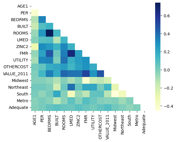
X_mat = owned_single_family_units_df4.drop(columns=["VALUE_2013", "METRO3", "REGION", "ZADEQ"])
X_mat = pd.concat([X_mat, dummies_df[['Midwest', 'Northeast', 'South', 'Metro', 'Adequate']]], axis=1)
# lower triangular matrix
mask2 = np.triu(np.ones_like(X_mat.corr()))
warnings.filterwarnings("ignore")
# plotting a triangle correlation heatmap
sns.heatmap(X_mat.corr(), cmap="YlGnBu", annot=True, fmt='0.1f', mask=mask2)
plt.savefig("corrMatrix.png");
y_resp = owned_single_family_units_df4["VALUE_2013"]
test_size = round(1000 / owned_single_family_units_df4.shape[0],4)
test_size
0.048
# Separate the data
X2_train, X2_test, y2_train, y2_test = train_test_split(X_mat, y_resp, test_size = test_size, random_state=42)
print("The number of samples in train set is {}".format(X2_train.shape[0]))
print("The number of samples in test set is {}".format(X2_test.shape[0]))
The number of samples in train set is 19821
The number of samples in test set is 1000
X2_train.to_csv("training_inputs.csv")
y2_train.to_csv("training_response.csv")
X2_test.to_csv("test_inputs.csv")
y2_test.to_csv("test_response.csv")
descriptive_stats = pd.concat([y2_train.describe(), X2_train.describe()], axis=1)
descriptive_statistics = descriptive_stats.rename(columns={"VALUE_2013": "ln_value_2013"})
descriptive_statistics.to_csv("descriptive_stats.csv")
# (1) Initiate the model
lr2 = LinearRegression()
# (2) Fit the model
lr2.fit(X2_train, y2_train)
# (3) Score the model
round(lr2.score(X2_test, y2_test),2)
0.61
params2 = np.append(lr2.intercept_, lr2.coef_)
params2
array([-4.15115916e+00,  8.47991382e-04, -8.45210427e-03, -3.93258886e-02,
        1.91488892e-03,  4.77613216e-02,  1.59614781e-01,  5.29324517e-02,
        3.69681281e-01,  5.34945627e-02,  7.14752260e-03,  5.83990141e-01,
       -9.61762889e-02, -7.98542103e-02, -1.07717874e-01, -4.43225115e-02,
        2.29460839e-02])
# Predict
y2_pred = lr2.predict(X2_test)
# Mean Square error
mse2 = metrics.mean_squared_error(y2_test, y2_pred)
print("Mean Squared Error {}".format(mse2))
Mean Squared Error 0.22820281510477217
pd.DataFrame(y2_pred).to_csv("predicted.csv")
# Mean Absolute Difference
round((np.abs(np.exp(y2_test) - np.exp(y2_pred))).mean())
72729
new_X2 = np.append(np.ones((len(X2_test), 1)), X2_test, axis=1)
new_X2[0]
array([1.00000000e+00, 3.90000000e+01, 5.00000000e+00, 4.00000000e+00,
       1.97000000e+03, 7.00000000e+00, 1.08573245e+01, 1.08546820e+01,
       6.85856503e+00, 6.12249281e+00, 4.60517019e+00, 1.14075649e+01,
       0.00000000e+00, 0.00000000e+00, 1.00000000e+00, 0.00000000e+00,
       1.00000000e+00])
# Varriance
v_b2 = mse2*(np.linalg.inv(np.dot(new_X2.T, new_X2)).diagonal())
# Standard error
se2 = np.sqrt(v_b2)
# t-statistics
t_b2 = params2/se2
# p-values
p_val2 = [2*(1 - stats.t.cdf(np.abs(i), (len(new_X2) - len(new_X2[0])))) for i in t_b2]
p_val2 = np.round(p_val2, 3)
p_val2
array([0.02 , 0.449, 0.508, 0.22 , 0.002, 0.002, 0.275, 0.002, 0.   ,
       0.189, 0.732, 0.   , 0.117, 0.168, 0.032, 0.251, 0.812])
warnings.filterwarnings("ignore")
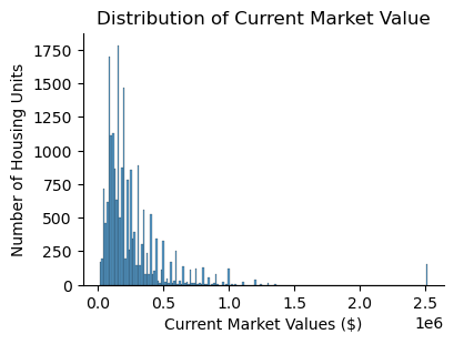
sns.displot(data=owned_single_family_units_df2, x='VALUE_2013', height=3, aspect=1.4, kde=False)
plt.xlabel("Current Market Values ($)")
plt.ylabel("Number of Housing Units")
plt.title("Distribution of Current Market Value")
plt.savefig("value2013.png")
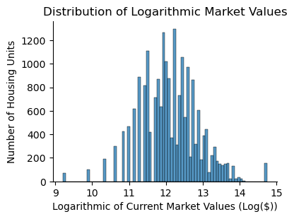
sns.displot(data=owned_single_family_units_df4, x='VALUE_2013', height=3, aspect=1.4, kde=False)
plt.title("Distribution of Logarithmic Market Values")
plt.xlabel("Logarithmic of Current Market Values (Log($))")
plt.ylabel("Number of Housing Units")
plt.savefig("logvalue2013.png");
# Let's first rename the features that were logarithmically transformed
X2_train.rename(columns={"VALUE_2011": "ln_value_2011", "UTILITY": "ln_utility", "OTHERCOST": "ln_othercost",
                         "LMED": "ln_lmed", "FMR": "ln_fmr", "ZINC2": "ln_zinc2"}, inplace = True)

coefs = pd.DataFrame(lr2.coef_, columns=["Coefficients"], index=X2_train.columns)

coefs_sorted = coefs.sort_values(by="Coefficients", key=abs, ascending=True)

coefs_sorted.plot(kind="barh", figsize=(9, 6))
plt.title("Multilinear Regression model - Feature Importance")
plt.axvline(x=0, color=".5")
plt.subplots_adjust(left=0.3)
plt.savefig("featureImportance.png")
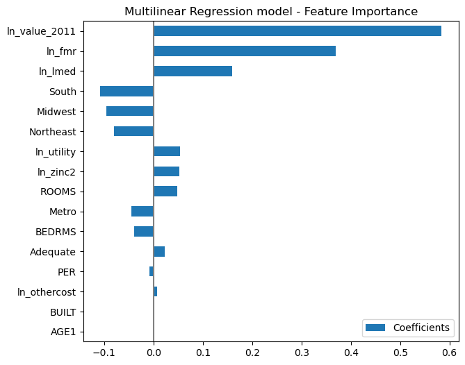
# Feature importance
coefs.sort_values(by="Coefficients", key=abs, ascending=False)
| Coefficients | |
|---|---|
| ln_value_2011 | 0.583990 |
| ln_fmr | 0.369681 |
| ln_lmed | 0.159615 |
| South | -0.107718 |
| Midwest | -0.096176 |
| Northeast | -0.079854 |
| ln_utility | 0.053495 |
| ln_zinc2 | 0.052932 |
| ROOMS | 0.047761 |
| Metro | -0.044323 |
| BEDRMS | -0.039326 |
| Adequate | 0.022946 |
| PER | -0.008452 |
| ln_othercost | 0.007148 |
| BUILT | 0.001915 |
| AGE1 | 0.000848 |
Interpretation of the Regression Coefficients
-
β0: No managerially relevant interpretation, since talking about a situation when all ‘X’ variables are zero does not make managerial sense.
-
β1: For every one percentage increase in the 2011 market value, the current market value increases by about 0.584%, all other variables being kept at the same level.
-
β2: For every one percentage increase in the fair market rent, the market value increases by 0.37%, all other variables remaining at the same level.
-
β3: For every one percentage increase in the area median income, the market value increases by 0.16%, all other variables remaining at the same level.
-
β4: When the housing unit is in the south region of the country, then the market value tends to be lower by 10.8% as compared to a similar housing unit being in the West region, all other variables being kept at the same level.
-
β5: When the housing unit is in the midwest region of the country, then the market value tends to be lower by 9.6% as compared to a similar housing unit being in the western region, all other variables being kept at the same level.
-
β6: When the housing unit is in the northeast region of the country, then the market value tends to be lower by 8.0% as compared to a similar housing unit being in the western region, all other variables being kept at the same level.
-
β7: For every one percentage increase in the monthly utility costs, the market value increases by 0.053%, all other variables remaining at the same level.
-
β8: For every one percentage increase in the annual household income, the market value increases by 0.053%, all other variables remaining at the same level.
-
β9: One additional room corresponds to a 4.8% increase in the market value of the housing unit, all other variables being kept at the same level.
-
β10: When the geographical location of the Housing unit is classified as a ‘Central City’ area, then the market value of the housing unit is lower by 4.4%, all other variables being kept at the same level.
-
β11: Every additional bedroom corresponds to a 4.0% decrease in the market value of the housing unit, all other variables being kept at the same level
-
β12: When the housing unit is classified as ‘Adequate’ as compared to other adequacy categorizations, then the market value tends to be higher by 2.3%, all other variables being kept at the same level.
-
β13: Every additional person in the household corresponds to a 0.8% decrease in the market value of the housing unit, all other variables being kept at the same level.
-
β14: For every one percentage increase in the monthly utility costs, the market value increases by 0.007%, all other variables remaining at the same level.
-
β15: Every one-year delay in the ‘Year Built’ of the housing unit, there is a 0.2% increase in the market value of the housing unit, all other variables being kept at the same level.
Interpretation of R-square
The R-square is about 0.61, indicating that the model explains about 61 percent of the variation in the market value of housing units.